Motives for Spending, Saving and Borrowing
The basic determinants of consumer spending and saving were covered as part of the AS course. In this section we delve deeper into the determinants of consumption exploring in particular the Keynesian approach and alternative theories of consumption and saving.
The consumption function
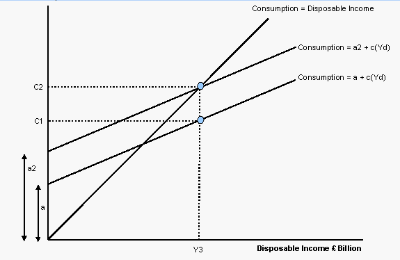
The consumption function is simply a theoretical relationship between income and consumer expenditure. The Keynesian theory describes a consumption function where household spending is directly linked to people’s disposable income. A simplified consumption function diagram is shown below.
The consumption function
The consumption function is simply a theoretical relationship between income and consumer expenditure. The Keynesian theory describes a consumption function where household spending is directly linked to people’s disposable income. A simplified consumption function diagram is shown below.
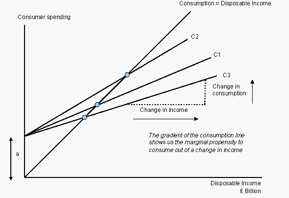
The standard Keynesian consumption function is written as follows:
C = a + c (Yd) - where
The key to understanding how a rise in disposable income affects household spending is to understand the concept of the marginal propensity to consume (mpc). The marginal propensity to consume is the change in consumer spending arising from a change in disposable income. If for example your disposable income rises by £5,000 and you choose to spend £3000 of this on extra goods and services, then the mpc is £3000/£50000 or 0.66. If you chose instead to spend only £2500 of the increase in income, then the mpc would be 0.5.
The gradient of the consumption function shown in the previous diagram is determined by the value formarginal propensity to consume. A change in the mpc (shown in the next diagram) would cause a pivotal change in the consumption function. For example, a decision to save less of any increase in income would lead to a rise in the mpc and a steeper consumption curve.
C = a + c (Yd) - where
- C is total consumer spending
- a is autonomous spending
- And c (Yd) is the propensity to spend out of disposable income
The key to understanding how a rise in disposable income affects household spending is to understand the concept of the marginal propensity to consume (mpc). The marginal propensity to consume is the change in consumer spending arising from a change in disposable income. If for example your disposable income rises by £5,000 and you choose to spend £3000 of this on extra goods and services, then the mpc is £3000/£50000 or 0.66. If you chose instead to spend only £2500 of the increase in income, then the mpc would be 0.5.
The gradient of the consumption function shown in the previous diagram is determined by the value formarginal propensity to consume. A change in the mpc (shown in the next diagram) would cause a pivotal change in the consumption function. For example, a decision to save less of any increase in income would lead to a rise in the mpc and a steeper consumption curve.
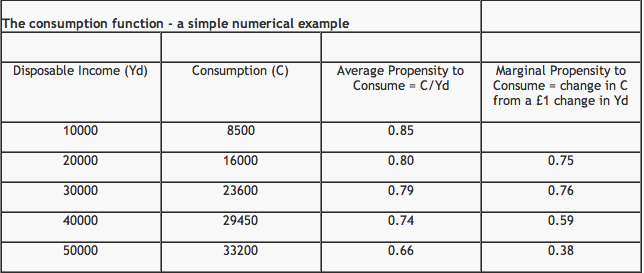
In our example above, as disposable income rises in blocks of £10,000, so does total consumption. But the rate at which consumer spending is increasing is declining. The marginal propensity to consume is falling and this brings down the average propensity to consume. The Keynesian theory did actually argue that the marginal propensity to consume would fall as income increases, but the evidence for the UK over many years disputes this.
The Savings Function
We assume that any disposable income that is not spent is saved, so we can deduce from our numerical example above, that because the marginal propensity to consume is falling, then the marginal propensity to save must be rising as is the average propensity to save (otherwise known as the household savings ratio).
This is shown in the table below which is drawn from the data on consumption and income used in the first table.
The savings ratio is quite volatile but what have been the main trends since 1990?
Looking at the data for the household savings ratio we find that it has been quite volatile over the last fifteen years ranging from over 13% of disposable income in 1992 to just 3% of disposable income in 2004. It is noticeable that in recent years, households have chosen to save a lower percentage of their after-tax income than in previous periods. Much of this has been the result of the boom in consumer borrowing, including a huge level of mortgage equity withdrawal from the housing market.
By the summer of 2005 it was clear that the borrowing boom was coming to an end in part the result of a sharp slowdown in the rate of growth of house prices. In the last couple of years there has been a steady rise in the savings ratio with its value heading up towards 6%. This has coincided with a period of weaker consumer demand for goods and services. People have obviously decided to save a little more in order to repay some debt and generally improve their household finances. Perhaps they fear rising unemployment and the risks of defaulting on their loans?
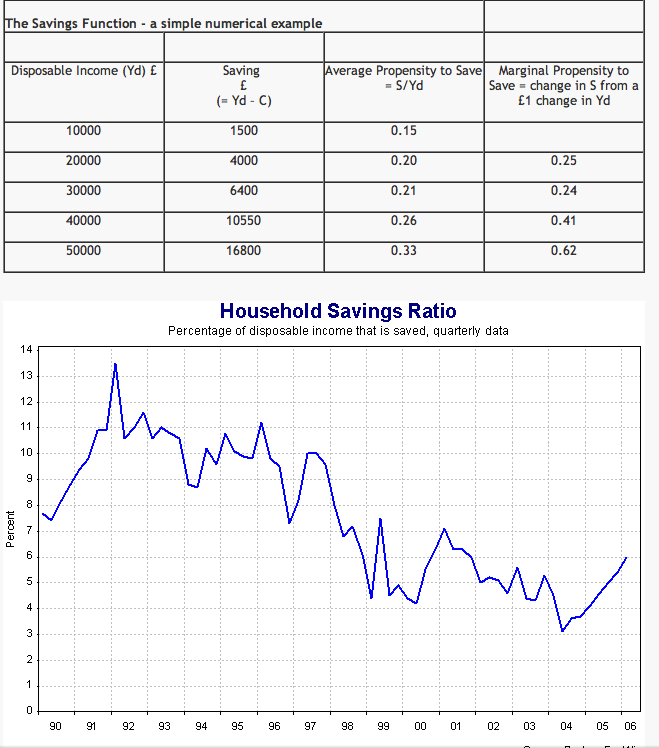
Unemployment and interest rates both influence savings decisions
In the chart above we track the household savings ratio, the base rate of interest set by the Bank of England and the seasonally adjusted rate of unemployment as measured by the claimant count. The general trend is that the savings ratio has declined over the last decade or more, a time when both unemployment and interest rates have also fallen. If people have reasonable expectations of job security and if the rate of return on their savings is lower than in the past, here are two reasons to save less and borrow more.
Notice in the next chart how the incredibly strong demand for consumer borrowing has tailed off in the last two years. The annual growth in demand for consumer credit exceeded 10% from 1994 through to the middle of 2005. The growth rate has since dipped sharply lower; perhaps our love affair with the plastic card (40 years old in 2006) is coming to an end? In contrast, the rate of increase in borrowing secured on the value of property has remained very strong. Borrowing money represents dis-saving because it allows someone to spend in excess of their current income.
The issue of consumer debt is a long-standing one. It certainly raises risks for the UK economy in the years ahead because the accumulation of debt creates the cost of servicing this debt, thousand of people have problems in simply paying the interest on their loans and the number of personal insolvencies in the UK has reached a record high.
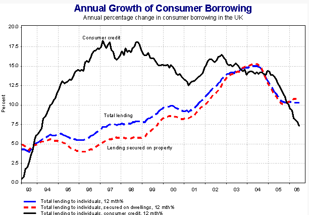
The last ten years has seen a credit boom in the UK – now coming to an end?
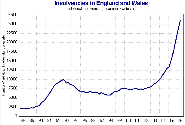
Personal insolvencies are now at a record high – too much borrowing? Or is it now too easy to declare oneself bankrupt and avoid repaying existing debts?
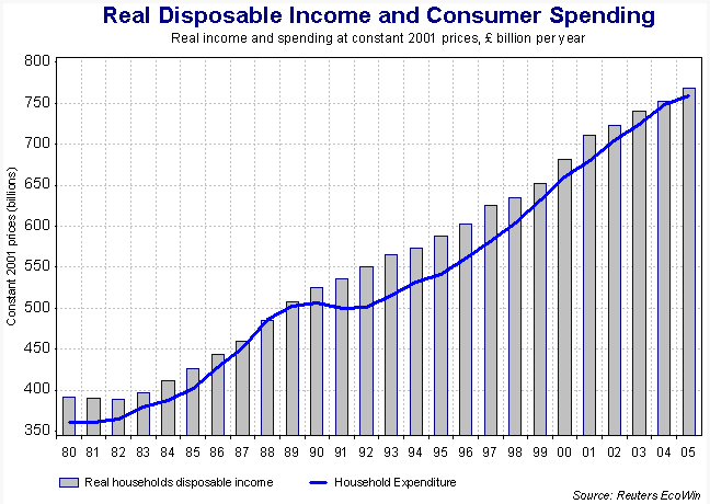
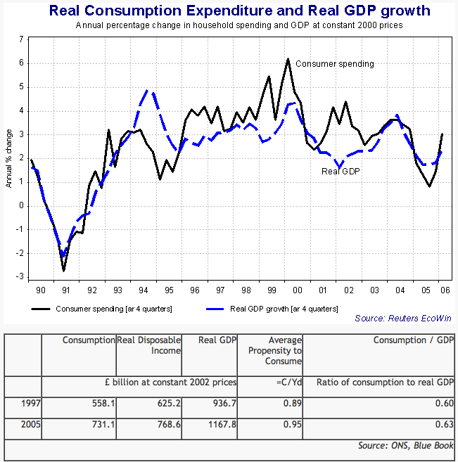
There is a strong relationship between people’s disposable income and their spending
Shifts in the Consumption Function
Shifts in the Consumption Function
A change in any factor affecting consumption other than a change in income is said to lead to a shift in the consumption function. These factors include the following:
- A change in interest rates – for example a cut in interest rates will boost consumption at each level of income and cause an upward shift in the consumption function. Lower interest rates act to lower the cost of servicing the debt on a mortgage and thereby increase the effective disposable income of homeowners. In contrast a period of higher interest rates is designed to curb consumer spending.
- A change in household wealth – for example a rise in house prices or in share prices encourages higher levels of borrowing and an upward movement in the consumption curve
- A change in consumer confidence – for example, expectations of rising unemployment and worsening expectations of changes in income might lead to a reduction in confidence and a fall in spending at each level of income. Conversely an improvement in consumer expectations about the health of the economy will increase confidence and planned spending
We now turn to some non-Keynesian theories of what determines consumer spending.
Alternative theories of consumption
The life—cycle model
The life-cycle model of consumption was developed by Franco Modigliani who argued that households form a view about their likely or expected income over a large slice of their life-cycle, and then base their spending decisions around this. This helps to explain why people in reasonably well paid jobs in their early twenties are prepared to borrow heavily to finance current consumption (a new car, furnishings for a property) because they expect to be able to repay loans as their disposable income increases. Similarly people reaching middle age frequently tend to become net savers because they are anticipating saving for their retirement. One of the results of the life-cycle model is that changes in the age structure of the population can have sizeable effects on total consumer spending in the economy.
The permanent income model
This model of consumption is associated with the US economist Milton Friedman and it is, in many ways, a development of the life-cycle mode. Friedman believed that people base their spending decisions on expectations of permanent income. Permanent income might be described as the average income that people can earn over their lifetime. A distinction is made between transitory income (e.g. a windfall gain in income which has not been earned) and permanent income. Friedman believed that changes in transitory income would not fundamentally affect spending and saving decisions. But that shifts in permanent income would be important in shaping our spending levels.
For example, a rise in household wealth increases the ability of people to spend perhaps through borrowing secured on the value of a property. Lower interest rates tend to increase both share and house prices adding to household wealth. That said lower interest rates also cut the income flowing to people with net savings.
According to the permanent income model, only changes in permanent income have any long term effect on consumption. But transitory changes in spending power can lead to a more volatile pattern for the propensity to consume.
Key Points
- Keynesian theories of consumption focus on current disposable income as the main determinant of household spending
- Other theories argue that expectations of income and wealth in the future also affect people’s spending decisions
- Borrowing allows people to spend more than their current income. Borrowing is dis-saving
- The consumer borrowing boom has lasted more than a decade
- Household debt is now at a record high although interest rates remain low by historical standards
- Rising house prices have boosted personal wealth and consumer confidence
- Personal insolvencies are rising, debt is likely to be a major constraint on consumer demand for goods and services in the years ahead
